Newtonian lift simulation on CUDA
Once I came across a rather curious article “Scientific and technical myths, part 1. Why do planes fly?” (Russian original). The article describes in detail what problems arise when one’s trying to explain lift using Bernoulli’s law or the Newtonian lift theory. Although the article offers other explanations, I still would like to talk about the Newtonian model in extra detail.
The general assumption of this model is the absence of interaction of gas particles with each other. Because of this, at standard conditions, it gives incorrect results, although it still can be used for some extreme conditions where the interaction can be omitted.
I decided to check what would happen in the Newtonian model if I add interatomic interaction to it. The source code and binaries of the resulting simulator are available on GitHub.
Before we dive deeper, I’d like to point out that this article is not about physics itself. It’s about GPGPU programming. We won’t discuss the physical properties of the model, because it’s known to be oversimplified and unsuitable for real case applications. Yet this imprecise model gives a more accurate and intuitive description of the phenomenon than Bernoulli’s law.
This text is the author’s translation of the original article.
Computational Fluid Dynamics
It’s a brief overview section. You can skip it because the simulation doesn’t use CFD methods.
Computational fluid dynamics (CFD) deals with the problems of the exact simulation of liquids and gases. It uses the Navier-Stokes equations because they describe liquids and gases surprisingly well.
If you are not familiar with these equations but would like to understand them, there is a very good derivation of them in The Feynman Lectures on Physics, Volume II. See chapters 38 (Elasticity), 40 (The Flow of Dry Water), and 41 (The Flow of Wet Water). Or you can just watch this short video by Numberphile.
The simplest system of the Navier-Stokes equations consists of two equations. The first one is the vector equation of Newton’s second law. This equation determines the resultant of all internal (pressure, viscosity) and external (gravity) forces. The second one is a continuity equation which denotes flow incompressibility. More advanced versions of the Navier-Stokes equations may also include additional conditions and equations.
Generally, the system can be solved in two different ways: the Lagrangian or Eulerian approaches. The Eulerian approach describes a fluid as a set of vector and scalar fields. The Lagrangian approach describes the fluid as a set of individual particles.
In the case of the Eulerian approach, there is a bunch of ways to solve the system numerically. For example, you can use the finite element method (FEM) or the finite volume method (FVM), in conjunction with the adaptive mesh refinement (see also Finite Element vs Finite Volume).
Why the adaptability of the grid is useful and how it can be implemented have been described in detail in the talk down below made by Adam Lichtl and Stephen Jones.
As far as I know, the Eulerian approach is usually applied to simulate closed volumes of continuous media, i.e., there are no empty spaces and inclusions of other media. It provides more accurate results thanks to its continuous nature. The Lagrangian approach is suitable for less precise simulations of non-continuous media. It’s most often implemented via the smoothed-particle hydrodynamics method (SPH) or more accurate the finite point method (FPM). The methods are actively used to simulate water with a full range of phenomena such as splashes, drops, puddles, surface wetting, etc. You can even include air particles into the simulation to simulate foam or bubbles. Reconstruction of the fluid surface can be done in any suitable way, such as screen-space meshes, dual contouring, marching tetrahedra, metaballs. If you know other interesting approaches, welcome to the comments below.
Discrete Element Method
My goal was to find an approach that would allow my simulator to calculate millions of particles in real-time.
The discrete element method (DEM) seemed very interesting to me because it solved almost a similar problem. However, it is primarily intended for modeling of granular media, where each particle has a position, orientation, arbitrary shape, and mass.
To reduce the complexity of the calculations, I decided to leave the particles only two degrees of freedom (X and Y coordinates), and keep the same mass and radius. For the sake of performance, I wanted to discard the parameters and factors that generate second-order effects. However, they can be very significant if complex systems are modeled. Here’s an illustrative example. NASA used the ideal gas model instead of the real gas one while designing the Space Shuttle. As a result, various reentry anomalies appeared during the STS-1 mission. You can read more in the Mission Anomalies section.
There’s one essential feature of DEM. It is discrete collision detection (DCD), i.e., collisions are processed a posteriori. It means particles may intersect each other or even go tunneling absolutely legally, a.k.a. “get stuck in textures”. The DCD method resolves collisions simply applying Hooke’s law force.
In contrast to this approach, there is an a priori method, the continuous collision detection method (CCD). It calculates the time point in the future when the collision only occurs. Knowing the exact contact time, the simulator alters the timestep to avoid intersections and tunneling. The method is actively used in modern games. For games, CCD is vital. Game objects must not tunnel through and intersect each other, so the player must not “get stuck in textures”. The method is supported by modern engines, by Unity and Unreal for sure.
Unfortunately, CCD has two major drawbacks. The first is the following: its accuracy costs lots of computational resources. Computations grow disproportionally as the number of objects increases. For a large number of particles, it would make the calculations completely impractical. As for the second one: when the density of particles increases, the mean free path of each one decreases. It forces the simulator to take smaller and smaller timesteps in order not to miss collisions. One of my projects suffers this effect significantly. It is seen very clearly how the timestep reduces to almost zero as the density of “planetary clumps” increases.
Therefore, for practical reasons, I decided to use DCD as an a posteriori method.
The cannonball effect
Having developed the first version of the simulation, I found that the particles hitting the front of the wing behave very familiarly. The leading edge of the wing pushes the molecules apart thanks to its drop-like shape. The reflected layer of particles creates a shockwave that reflects the following layer. And it, in its turn, affects the next layer and so on.
I’ve heard of a similar effect in a National Geographic documentary. It said that this phenomenon was exploited directly by the designers of the Space Shuttle. They made the nose of the Shuttle blunt deliberately. At high speeds, it created a shockwave that protected the protruding parts of the fuselage from destructive hot plasma.

In the documentary, this effect was compared to a cannonball. Flying far is not the goal of a cannonball, but striking is. Cannonballs don’t have to be aerodynamic. Thanks to this effect the blunt nose of the Shuttle protects the entire vessel so well. More details are available on the link with the timecode: https://youtu.be/v1_WqVguRJg?t=2497
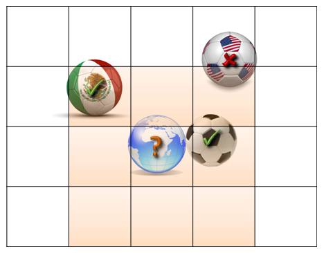
Surprisingly, this very effect is perfectly observed in the simulation. Probably, this cannonball effect of the interaction of the air layers along with the angle of attack gives the lift. The pressure heatmap below shows clearly the high (red and orange) and low (green and blue) pressure areas. The presence of interactions between particles has made the oversimplified Newtonian model much more interesting.


Simulator architecture
Let’s now have a look at how the simulator works. The application consists of two independent modules:
- The renderer of the current state.
- The simulation module on CPU or CUDA.
The modules are loosely coupled to each other and do not directly depend on each other. It is possible to simulate offline and render the results later. In the CUDA version of the demo, the rendering occurs every 16 steps as it is shown in the video at the beginning of the article.
Phase space
The concept of phase space is widely used in various kinds of simulations. The basic idea is that all variables of the system, such as position, orientation, momenta, etc., are packed into one large vector. This multidimensional vector denotes a point in the so-called phase space. The simulation itself is nothing more than the movement of a point through this space.
This form is very convenient because almost any simulation can be expressed like this. The movement of a state point is typically expressed in terms of an ordinary differential equation (ODE). Any ODE looks like the one below.
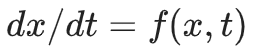
Here x is the position of the point (state) in the multidimensional phase space, and f is a black-box function. The function simply returns the instant velocity of the point. If we know the instant velocity we can then predict the next position like this:
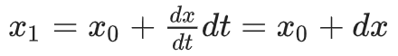
Regardless of how f works, the simulation is just a numerical integration process.
To know more about the phase space concept read the “Differential Equation Basics” and “Particle Dynamics” sections of the course: https://www.cs.cmu.edu/~baraff/sigcourse/
Great stuff is also available on the 3Blue1Brown channel

Integrator
After various experiments with numerical integrators, I decided to stick to the roughest, but at the same time the simplest the forward Euler method. I had also tried to use the 4th order Runge-Kutta (RK4) method, including the adaptive timestep algorithm. The major advantage of RK4 is that it allows us to make huge timesteps at quite a reasonable cost of a fourfold increase in computation. But in my case, it turned out that my model required small timesteps because I needed to avoid tunneling particles through each other. If you want to know more about how adaptive time step integrators work based on error assessment you can read “Differential Equation Basics” lecture notes, section 3, “Adaptive Stepsizes”.
In this simulation, to keep tunneling at a minimum, step adaptability is achieved by the following heuristic rule. The simulator finds the fastest particle and calculates the time it takes for this particle to travel its radius distance. This estimation is used as a timestep for the current iteration.
State derivate computation
Now let’s move on to the core of the simulator. Let’s look at the implementation of function f I have mentioned in the section “Phase space”. There is a high-level derivative solver code for the CPU and CUDA versions down below. I should point out that the CPU version had been developed before the CUDA one since it was easier to debug math in it. I added some improvements and optimizations in the CUDA version, but the idea remained the same. The difference is in the reordering of the particles. Read more in the “Particle Reordering” section.
//CPU version
void CDerivativeSolver::Derive(const OdeState_t& curState, OdeState_t& outDerivative)
{
    ResetForces();
    BuildParticlesTree(curState);
    ResolveParticleParticleCollisions(curState);
    ResolveParticleWingCollisions(curState);
    ParticleToWall(curState);
    ApplyGravity();
    BuildDerivative(curState, outDerivative);
}//CUDA version
void CDerivativeSolver::Derive(const OdeState_t& curState, OdeState_t& outDerivative)
{
    BuildParticlesTree(curState);
    ReorderParticles(curState);
    ResetParticlesState();
    ResolveParticleParticleCollisions();
    ResolveParticleWingCollisions();
    ParticleToWall();
    ApplyGravity();
    BuildDerivative(curState, outDerivative);
}
Finding collisions between particles
You may have already guessed by now that collision detection is the most computational intensive calculation. In the video at the very beginning of the article, 2'097'152 particles are involved. Among all this quantity, the simulation must somehow find all the colliding pairs quickly. Interestingly, this problem does not have a uniquely correct solution. Any method is a set of trade-offs and assumptions.
One of the possible options is to use a uniform grid structure, i.e., a grid of cells similar to a checkerboard. One of the GPU implementations is described in “Chapter 32. Broad-Phase Collision Detection with CUDA”.
In this case, the search for collisions takes about O(1) on average, which is extremely good. Each particle needs to traverse the lists in 9 (3x3) or 27 (3x3x3) cells for 2D or 3D cases respectively. Another advantage of the structure is the relative simplicity of parallelizing its construction. Memory for lists can be allocated either in advance in the form of an array, and the output index can be calculated through atomic increments, or a classic RCU lock-free singly-linked list can be built. Nvidia added heap support to its graphics cards a long time ago, so you can call malloc() / free() right in the device code, allocating and freeing list items.
This structure however may run into the following restrictions:
- The set of coordinate values is limited by the size of the grid itself. The restriction may be relaxed though by applying the modulo-like operation to the coordinate, i.e., by wrapping the flat space into a torus.
- Close cells in Euclidean space are usually located far away in the RAM / VRAM address space, without sharing a single cache line, which creates an additional load on the memory bus.
- If there’s a low density of objects or a small number of them, the data structure consumes more memory than the data itself.
- Excessively long lists may appear with a high density of objects.
- Due to the hardware features of GPU thread scheduling, some lock-free structures don’t work correctly (https://youtu.be/86seb-iZCnI?t=2311, link with timecode).
Fortunately, there’s another intriguing option. We can build a BVH-tree based on the Z-order curve (a.k.a. Morton curve, Morton codes). I stumbled upon this rather curious data structure while I was looking for alternatives to the uniform grid.
The Z-order curve is a space-filling fractal curve.
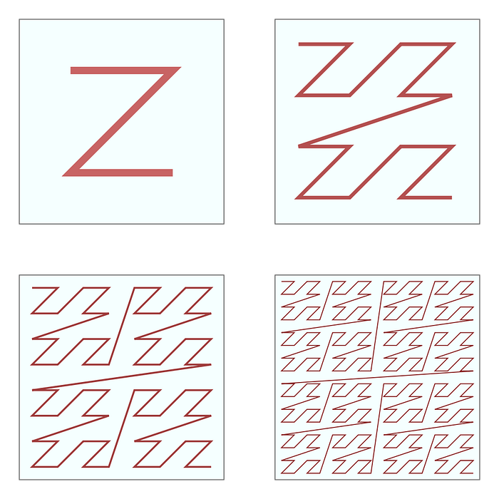
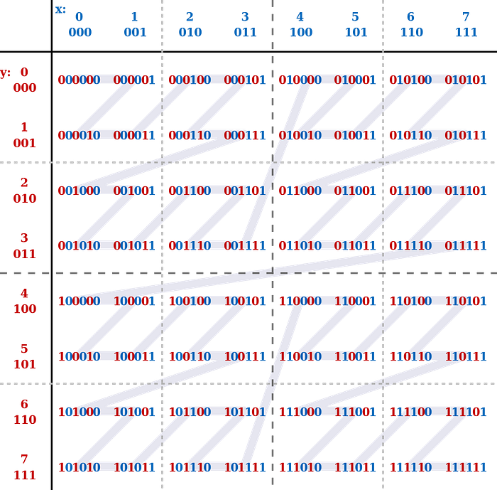
As a space-filling curve, the Z-order curve folds a high-dimensional space into a single dimension. Interestingly, if we sort objects by index on the curve, we may notice that a set of objects located close to each other in Euclidian space, generally, is also close in one-dimensional space. This property can significantly increase the memory bus bandwidth if we order particles this way. By the way, if you need to do image processing you might want to store pixels as one of these curves, rather than a matrix.
One more interesting feature of this data structure is that the building edges between tree nodes may be performed in parallel. During the process of linking, threads do not need to communicate with each other in any way. It allows us to achieve the maximum level of parallelism. This approach has been proposed by the engineer Tero Karras from Nvidia. He has designed this method specifically for solving the problem of finding collisions on the GPU.
A brief description of the algorithm:
- Tree traversal: https://developer.nvidia.com/blog/thinking-parallel-part-ii-tree-traversal-gpu/
- Tree construction: https://developer.nvidia.com/blog/thinking-parallel-part-iii-tree-construction-gpu/
The detailed description is available here: https://developer.nvidia.com/blog/wp-content/uploads/2012/11/karras2012hpg_paper.pdf
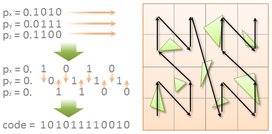
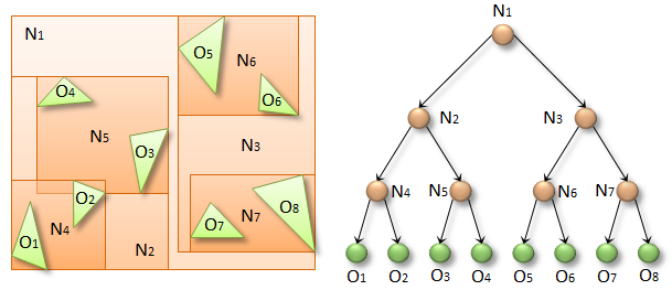
Long story short, the algorithm is as follows. For each of the N objects, N threads get launched. Each thread calculates the bounding box of each object and, based on its center, calculates the Morton code (index on the Z-curve). After this step, the boxes are sorted in ascending order by the code value.
Then the tree nodes initialization occurs. Before we build the tree, it is known beforehand that for N leaves there are N-1 intermediate nodes. Accordingly, all necessary memory allocations and initial initializations occur at this step.
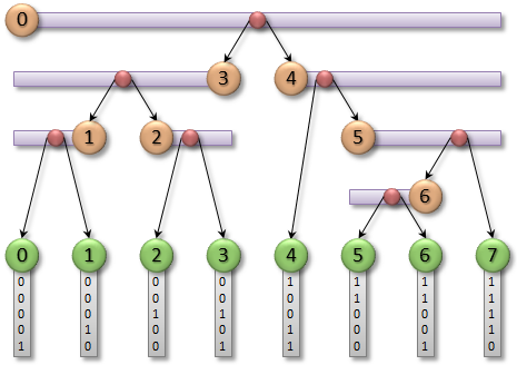
And here is the most sophisticated stage. We need to find a difference in bits between two neighbor codes, moving from the most significant bit to the least significant one. The presence of a difference signals that an intermediate node must be formed. The figures below show the single-threaded and parallelized versions of the algorithm.
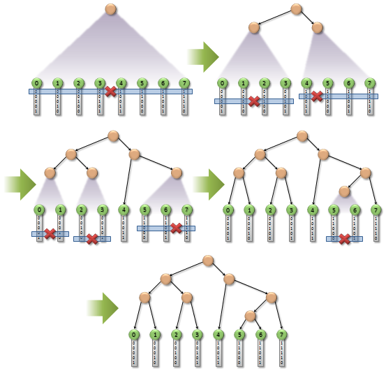
There are some special cases in the parallel algorithm, so please refer to the original paper to know more.
When we are done building the edges, we may proceed to the BVH-structure construction.
N threads start from leaves and, going up to the root, update the boxes of intermediate nodes. Since it is undefined which of the children will come to the parent first, a special atomic flag is stored in the intermediate nodes, which is initially set to zero. Both children use the atomicExch() function to set the flag to 1. The function returns the value before the modification. The child has come to the parent first if the function has returned 0. This also means that the current thread cannot modify the parent’s box, because the box of the sibling may not be ready yet. At this point, the thread ends its execution. If the function has returned 1, therefore the child can safely modify the parent’s box, combining the boxes of both siblings, and repeat the process again.
After this stage, the tree is ready for traversal.
Collision response
There are two types of collisions responses in the simulation: “particle-to-particle” and “particle-to-airfoil”.
The “particle-to-particle” response exploits the fact that the objects are already stored in the tree. There is a special procedure for “reflexive” or self-traversal where leaves look for collisions with each other. This optimized procedure has been introduced by Tero Karras. The idea is that the procedure must recognize A-B and B-A collisions as the same collision, so it is detected only once. To do this, additional information is stored while the tree is being built. The intermediate nodes store the index of the rightmost leaf that can be reached out of the node. For example, in the figure above, the rightmost leaf of N2 is O4, and the rightmost one of N3 is O8. When the thread associated with the leaf, let’s say O6, descends from the root, at some point it will refer to the intermediate node N2. Thanks to the rightmost value, it will detect that the O6 leaf is unreachable from the N2 subtree. In this case, the O6 thread should ignore the entire subtree N2. On the other hand, the threads associated with leaves from the N2 subtree must check the N3 subtree. Ultimately, if a collision with O6 exists, then only one thread will report it.
For the special case “reflexive” traversal procedure, the function prototype looks like this:
template<typename TDeviceCollisionResponseSolver>
void CMortonTree::TraverseReflexive(const TDeviceCollisionResponseSolver& solver);
For the case of “particle-to-airfoil”, a more common version is used.
template<typename TDeviceCollisionResponseSolver>
void CMortonTree::Traverse(const thrust::device_vector<SBoundingBox>& objects, const TDeviceCollisionResponseSolver& solver);
Here TDeviceCollisionResponseSolver is an object that should implement the following interface:
struct Solver
{
    struct SDeviceSideSolver
    {
        ...
        __device__ SDeviceSideSolver(...);
        __device__ void OnPreTraversal(TIndex curId);
        __device__ void OnCollisionDetected(TIndex leafId);
        __device__ void OnPostTraversal();
    };
    Solver(...);
    __device__ SDeviceSideSolver Create();
};
For each N object or each leaf in the case of a reflexive traversal, N threads get launched. Each thread creates its own solver via the Create() factory method. Then the OnPreTraversal() method gets called receiving the index of the current object. If the bounding box of the current object has overlapped the box of another leaf, the OnCollisionDetected() function gets called with the index of the other leaf as an argument. This function computes the collision response itself. After traversing the tree, OnPostTraversal() gets called.
This collision response protocol isn’t the first I got. From the beginning, I implemented it differently. I divided the tree traversal and physics computation into two different stages, as Tero Karras had done. However, I ran into the problem of building lists of the detected collisions. I tried storing information about collisions in the form of a N*O matrix, where N is the number of objects, O is the maximum size of the list. But I gave up on this idea because, in certain scenarios, space was quickly running out of the lists. And this, in turn, was creating various physical artifacts. In addition, I noticed that the profiler was signaling about inefficient memory usage (coalesced memory access). So I decided to try the no-list approach described above. To my surprise, the method turned out to be a little faster and provided no artifacts.
struct SParticleParticleCollisionSolver
{
  struct SDeviceSideSolver
  {
    CDerivativeSolver::SIntermediateSimState& simState;
    TIndex curIdx;
    float2 pos1;
    float2 vel1;
    float2 totalForce;
    float totalPressure;    __device__ SDeviceSideSolver(
      CDerivativeSolver::SIntermediateSimState& state) :
        simState(state)
    {    }    __device__ void OnPreTraversal(TIndex curLeafIdx)
    {
      curIdx = curLeafIdx;
      pos1 = simState.pos[curLeafIdx];
      vel1 = simState.vel[curLeafIdx];
      totalForce = make_float2(0.0f);
      totalPressure = 0.0f;
    }    __device__ void OnCollisionDetected(TIndex anotherLeafIdx)
    {
      const auto pos2 = simState.pos[anotherLeafIdx];
      const auto deltaPos = pos2 - pos1;
      const auto distanceSq = dot(deltaPos, deltaPos);
      if (distanceSq > simState.diameterSq || distanceSq < 1e-8f)
          return;      const auto vel2 = simState.vel[anotherLeafIdx];      auto dist = sqrtf(distanceSq);
      auto dir = deltaPos / dist;
      auto springLen = simState.diameter - dist;      auto force = SpringDamper(dir, vel1, vel2, springLen);
      auto pressure = length(force);
      totalForce += force;
      totalPressure += pressure;      atomicAdd(&simState.force[anotherLeafIdx].x, -force.x);
      atomicAdd(&simState.force[anotherLeafIdx].y, -force.y);
      atomicAdd(&simState.pressure[anotherLeafIdx], pressure);
    }    __device__ void OnPostTraversal()
    {
      atomicAdd(&simState.force[curIdx].x, totalForce.x);
      atomicAdd(&simState.force[curIdx].y, totalForce.y);
      atomicAdd(&simState.pressure[curIdx], totalPressure);
    }
  };  CDerivativeSolver::SIntermediateSimState simState;
  SParticleParticleCollisionSolver(
    const CDerivativeSolver::SIntermediateSimState& state) :
    simState(state)
  {
  }
  __device__ SDeviceSideSolver Create()
  {
      return SDeviceSideSolver(simState);
  }
};void CDerivativeSolver::ResolveParticleParticleCollisions()
{
  m_particlesTree.TraverseReflexive<SParticleParticleCollisionSolver>(SParticleParticleCollisionSolver(m_particles.GetSimState()));
    CudaCheckError();
}
During debugging, I have noticed that at high particle density, the OnCollistionDetected() function is usually called with the same arguments among the threads of the same warp. A typical scenario was the following: if in some region of space there were particles A, B, C, and D, which were in this order on the Z-curve, then something like that happened:
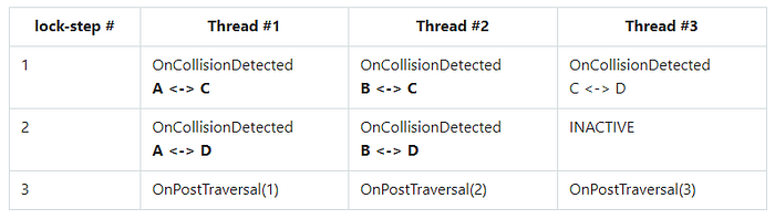
As you can see from the table, at steps 1 and 2, threads #1 and #2 performed atomicAdd() calls with the same particles C and D correspondingly while the OnCollistionDetected() function was running. This creates an additional workload for the atomic pipeline.
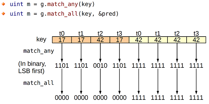
Starting with the Volta architecture, Nvidia has added support of new warp-vote instructions to the chips. Using the match_any instruction, a thread can examine the entire warp, getting a bitmask of threads for which the value of the requested variable is the same.
Communication inside the warp has also become more convenient because new warp shuffle functions have been added with support for thread masks.
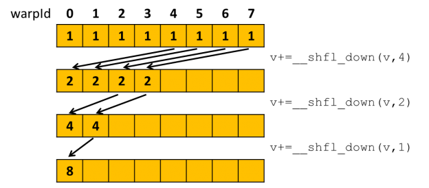
Thanks to these functions, threads can group by a common output address before accessing the global memory. Further, this group must perform the summation at the level of the Streaming Multiprocessor (SM) registers, and after that, only a single thread accesses the global memory. Unfortunately, there are no such instructions on my home 1080 Ti (Pascal), so I decided to try to emulate them. Alas, the emulation has not given any increase, as well as any slowdown. Profiling has shown that although the workload of the atomic pipeline has dropped significantly, the arithmetic workload has increased as well as the registers count per thread. For me, it was not possible to develop the simulator using chips with Volta or Turing. Although, I have managed to test the simulation on my buddy’s RTX 2060 and find a bug related to the atomic operation. About the bug read more in the “The memory barrier” section.
Other optimizations and remarks
In this section, I would like to talk about some of the differences from the original algorithm, which gave an additional increase in performance, as well as some remarks about this implementation.
SoA
“Structure of Arrays” is a technique that allows one to speed up memory access in certain situations.
When working with a tree at any stage the full set of node attributes is not usually required. So instead of storing each node as a structure, the entire tree is stored as SoA:
typedef uint32_t TIndex;struct STreeNodeSoA
{
  const TIndex leafs;  int* __restrict__ atomicVisits;
  TIndex* __restrict__ parents;
  TIndex* __restrict__ lefts;
  TIndex* __restrict__ rights;
  TIndex* __restrict__ rightmosts;
  SBoundingBox* __restrict__ boxes;
  const uint32_t* __restrict__ sortedMortonCodes;
};
The same applies to the internal state of the state derivative solver:
struct SIntermediateSimState
{
    const TIndex particles;
    const float particleRad;
    const float diameter;
    const float diameterSq;    float2* __restrict__ pos;
    float2* __restrict__ vel;
    float2* __restrict__ force;
    float* __restrict__ pressure;
};
At the same time, it makes no sense to store an array of bounding boxes in the SoA style, because both min and max points are required in all scenarios. Therefore, boxes are stored in “Array of Structures” (AoS) fashion:
struct SBoundingBox
{
  float2 min;
  float2 max;
};struct SBoundingBoxesAoS
{
  const size_t  count;
  SBoundingBox* __restrict__ boxes;
};
Particle reordering
Since the current implementation does not build collision lists but resolves collisions right in place, the following problem arises. After assigning Morton codes to the box centers, the boxes themselves get sorted. But the rest of the particle parameters remain unsorted. If we continue to access the data in the original order, we get uncoalesced memory access.
This access pattern is very slow on the GPU. To restore the coalesced memory access, the positions and velocities of the particles are also ordered along the curve. And after performing all the calculations, forces and pressure as output values return to their original order. The idea is not new and was borrowed from the already mentioned SpaceX talk: https://youtu.be/vYA0f6R5KAI?t=1939 (link with timecode).

This optimization gives a 50% performance increase: from 8 FPS to 12 FPS for two million particles.
Traversal stack in Shared Memory
The original article provides an example implementation where the stack for tree traversal is implemented as a local array in a function scope. The problem with this approach is that it uses thread-local memory, a region in global memory. This means that SM begins to perform long read and write transactions, which, among other things, may still be uncoalesced. The essence of this optimization is to use the superfast Shared Memory region in the Streaming Multiprocessor chip.
Here’s the original code:
__device__ void traverseIterative(
    CollisionList& list,
    BVH& bvh,
    AABB& queryAABB,
    int queryObjectIdx)
{
    // Allocate traversal stack from thread-local memory,
    // and push NULL to indicate that there are no postponed nodes.
    NodePtr stack[64]; //local-memory stack
    ...
}
And here’s my implementation with the shared memory stack:
template<
  typename TDeviceCollisionResponseSolver,
  size_t kTreeStackSize,
  size_t kWarpSize = 32>
__global__ void TraverseMortonTreeKernel(
  const CMortonTree::STreeNodeSoA treeInfo,
  const SBoundingBoxesAoS externalObjects,
  TDeviceCollisionResponseSolver solver)
{
  const auto threadId = blockIdx.x * blockDim.x + threadIdx.x;
  if (threadId >= externalObjects.count)
      return;  const auto objectBox = externalObjects.boxes[threadId];
  const auto internalCount = treeInfo.leafs - 1;  //shared-memory stack
  __shared__ TIndex stack[kTreeStackSize][kWarpSize];  unsigned top = 0;
  stack[top][threadIdx.x] = 0;  auto deviceSideSolver = solver.Create();
  deviceSideSolver.OnPreTraversal(threadId);  while (top < kTreeStackSize) //top == -1 also covered
  {
    auto cur = stack[top--][threadIdx.x];    if (!treeInfo.boxes[cur].Overlaps(objectBox))
      continue;    if (cur < internalCount)
    {
      stack[++top][threadIdx.x] = treeInfo.lefts[cur];
      if (top + 1 < kTreeStackSize)
        stack[++top][threadIdx.x] = treeInfo.rights[cur];
      else
        printf("stack size exceeded\n");      continue;
    }    deviceSideSolver.OnCollisionDetected(cur - internalCount);
  }  deviceSideSolver.OnPostTraversal();
}
Using shared memory has allowed me to achieve a 43% increase: from 14 FPS to 20 FPS. You can read more about the available memory types in the official documentation:
The memory barrier
When I was developing the simulator, I used only 1080 Ti, a Pascal-based GPU. Unfortunately, I had no opportunity to use another GPU for development purposes. But I had a chance to ask three friends of mine to run the application on their gaming laptops with the new at that time 20-series chips. All three laptops produced images with the artifacts in the figure below.

At first, I thought it was a rendering issue but couldn’t find the error anywhere. Checking the code of the simulation also yielded no results. Six months later I got the insight after watching this talk:
Half of the talk is devoted to the idea of memory barriers and why they are important when working with atomic-operations and lock-free structures. The importance comes out of the fact that processors tend to reorder the instructions (Out-of-order execution) maintaining the dependencies between them to ensure correctness. In the case of lock-free structures for processors, the dependence is not obvious to the processor. Therefore, memory barriers are needed to tell the processor that instructions reordering must be limited in some way. Each platform implements memory barriers differently, but fortunately, the C ++ standard developers have managed to build the most general model. A detailed description of each barrier semantics is available in the std::memory_order documentation.
The code down has two comments related to the memory barrier.
__device__ void CMortonTree::STreeNodeSoA::BottomToTopInitialization(size_t leafId)
{
  auto cur = leafs - 1 + leafId;
  auto curBox = boxes[cur];  while (cur != 0)
  {
    auto parent = parents[cur];
    //1. Beware! Here comes an atomic operation!
    auto visited = atomicExch(&atomicVisits[parent], 1);
    if (!visited)
      return;    TIndex siblingIndex;
    SBoundingBox siblingBox;    TIndex rightmostIndex;
    TIndex rightmostChild;    auto leftParentChild = lefts[parent];
    if (leftParentChild == cur)
    {
      auto rightParentChild = rights[parent];
      siblingIndex = rightParentChild;
      rightmostIndex = rightParentChild;
    }
    else
    {
      siblingIndex = leftParentChild;
      rightmostIndex = cur;
    }    siblingBox = boxes[siblingIndex];
    rightmostChild = rightmosts[rightmostIndex];    SBoundingBox parentBox = SBoundingBox::ExpandBox(curBox,
                                                 siblingBox);
    boxes[parent] = parentBox;
    rightmosts[parent] = rightmostChild;    cur = parent;
    curBox = parentBox;    //This memory barrier will protect you!
    //At the next iteration, this thread is guaranteed to see
    //all writes made by the neighbor threads.
    __threadfence();
  }
}
My mistake was that I did not use any memory barriers in the code that builds the BVH-tree, but at the same time actively uses the atomic flag. Interestingly, the original implementation doesn’t use any barriers either. Most likely, in addition to the new SIMT model (Volta SIMT Model and Starvation-Free Algorithms sections), Nvidia added more aggressive “out-of-order execution” algorithms to the new architectures starting with Volta. As a consequence, writes that should have been performed before atomicExch(), i.e., at the previous iteration of the loop, occurs after on “Turing”. As a result of such aggressive reordering of instructions, the second child, coming to the parent, sees that its sibling has already calculated and saved the bounding box in the global memory, but in fact not. The result is a data race.
thrust::device_vector
I noticed too late that thurst::device_vector works in a synchronous manner. In the constructor and in the resize() method, this container performs full synchronization with the GPU via cudaDeviceSynchronize(). Apparently, the developers were guided by the following reasoning. Since the vector is on the GPU, then the element constructors must also be called on the device. But since constructors can throw exceptions, you need to wait for their execution to catch all of them. The only available way for the library developers to transfer exceptions from the device to the host is full synchronization. Another issue I have discovered is the reduction algorithm (reduce, sum, min, max) is also synchronous since it returns the result to the host. Cuda UnBound Library (CUB) is free of this flaw. By the way, it has recently become a part of the thrust library as a backend, although earlier it had to be downloaded separately.
Profiling results
Finally, here is a detailed report of what is happening during the calculation of each step for two million particles.

Conclusion
When I started this project, I just wanted to use my GPU as a mini-supercomputer to test the Newtonian lift model. As a result, the task has turned out to be much more interesting and fruitful than expected. The simulation has unveiled a “cannonball effect”, and the work on the project itself resulted in quite a research.
I hope that the experience described in this article, as well as the proposed solutions to the problems, will help you in your projects, even if they are not related to the GPU.
If you would like to start learning CUDA but don’t know where to start, there is a great course on Youtube from Udacity “Intro to Parallel Programming”. I recommend reviewing. https://www.youtube.com/playlist?list=PLAwxTw4SYaPnFKojVQrmyOGFCqHTxfdv2
Finally, a few more video simulations: